Shadertoy Tutorial Part 6 - 3D Scenes with Ray Marching

Greetings, friends! It's the moment you've all been waiting for! In this tutorial, you'll take the first steps toward learning how to draw 3D scenes in Shadertoy using ray marching!

Introduction to Rays

Have you ever browsed across Shadertoy, only to see amazing creations that leave you in awe? How do people create such amazing scenes with only a pixel shader and no 3D models? Is it magic? Do they have a PhD in mathematics or graphics design? Some of them might, but most of them don't!

Most of the 3D scenes you see on Shadertoy use some form of a ray tracing or ray marching algorithm. These algorithms are commonly used in the realm of computer graphics. The first step toward creating a 3D scene in Shadertoy is understanding rays.

Behold! The ray! 🙌

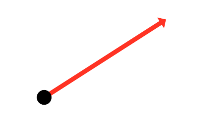
That's it? It looks like a dot with an arrow pointing out it. Yep, indeed it is! The black dot represents the ray origin, and the red arrow represents that it's pointing in a direction. You'll be using rays a lot when creating 3D scenes, so it's best to understand how they work.

A ray consists of an origin and direction, but what do I mean by that?

A ray origin is simply the starting point of the ray. In 2D, we can create a variable in GLSL to represent an origin:

vec2 rayOrigin = vec2(0, 0);

You may be confused if you've taken some linear algebra or calculus courses. Why are we assigning a point as a vector? Don't all vectors have directions? Mathematically speaking, vectors have both a length and direction, but we're talking about a vector data type in this context.

In shader languages such as GLSL, we can use a vec2 to store any two values we want in it as if it were an array (not to be confused with actual arrays in the GLSL language specification). In variables of type vec3, we can store three values. These values can represent a variety of things: color, coordinates, a circle radius, or whatever else you want. For a ray origin, we have chosen our values to represent an XY coordinate such as (0, 0).

A ray direction is a vector that is normalized such that it has a magnitude of one. In 2D, we can create a variable in GLSL to represent a direction:

vec2 rayDirection = vec2(1, 0);

By setting the ray direction equal to vec2(1, 0), we are saying that the ray is pointing one unit to the right.

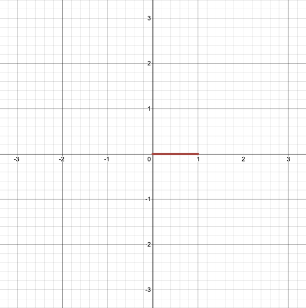
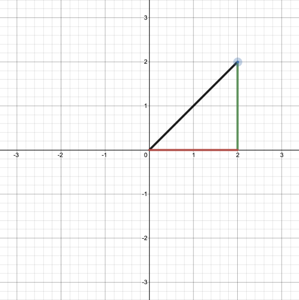
2D vectors can have an x-component and y-component. Here's an example of a ray with a direction of vec2(2, 2) where the black line represents the ray. It's pointing diagonally up and to the right at a 45 degree angle from the origin. The red horizontal line represents the x-component of the ray, and the green vertical line represents the y-component. You can play around with vectors using a graph I created in Desmos.

This ray is not normalized though. If we find the magnitude of the ray direction, we'll discover that it's not equal to one. The magnitude can be calculated using the following equation for 2D vectors:

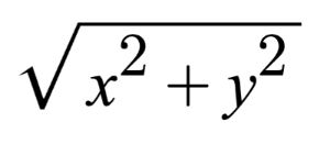
Let's calculate the magnitude (length) of the ray, vec2(2,2).

length(vec2(2,2)) = sqrt(x^2 + y^2) = sqrt(2^2 + 2^2) = sqrt(4 + 4) = sqrt(8)

The magnitude is equal to the square root of eight. This value is not equal to one, so we need to normalize it. In GLSL, we can normalize vectors using the normalize function:

vec2 normalizedRayDirection = normalize(vec2(2, 2));

Behind the scenes, the normalize function is dividing each component of the vector by the magnitude (length) of the vector.

Given vec2(2,2):
x = 2
y = 2

length(vec2(2,2)) = sqrt(8)

x / length(x) = 2 / sqrt(8) = 1 / sqrt(2) = 0.7071 (approximately)
y / length(y) = 2 / sqrt(8) = 1 / sqrt(2) = 0.7071 (approximately)

normalize(vec2(2,2)) = vec2(0.7071, 0.7071)

After normalization, it looks like we have the new vector, vec2(0.7071, 0.7071). If we calculate the length of this vector, we'll discover that it equals one.

We use normalized vectors to represent directions as a convention. Some of the algorithms we'll be using only care about the direction and not the magnitude (or length) of a ray. We don't care how long the ray is.

If you've taken any linear algebra courses, then you should know that you can use a linear combination of basis vectors to form any other vector. Likewise, we can multiply a normalized ray by some scalar value to make it longer, but it stays in the same direction.

3D Euclidean Space

Everything we've been discussing about rays in 2D also applies to 3D. The magnitude or length of a ray in 3D is defined by the following equation.

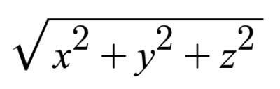
In 3D Euclidean space (the typical 3D space you're probably used to dealing with in school), vectors are also a linear combination of basis vectors. You can use a combination of basis vectors or normalized vectors to form a new vector.

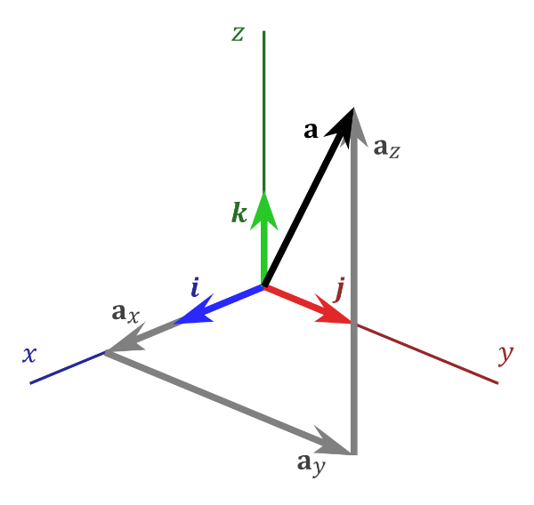
In the image above, there are three axes, representing the x-axis (blue), y-axis (red), and z-axis (green). The vectors, i, j, and k, represent fundamental basis (or unit) vectors that can be combined, shrunk, or stretched to create any new vector such as vector a that has an x-component, y-component, and z-component.

Keep in mind that the image above is just one portrayal of 3D coordinate space. We can rotate the coordinate system in any way we want. As long as the three axes stay perpendicular (or orthogonal) to each other, then we can still keep all the vector arithmetic the same.

In Shadertoy, it's very common for people to make a coordinate system where the x-axis is along the horizontal axis of the canvas, the y-axis is along the vertical axis of the canvas, and the z-axis is pointing toward you or away from you.

Notice the colors I'm using in the image above. The x-axis is colored red, the y-axis is colored green, and the z-axis is colored blue. This is intentional. As mentioned in Part 1 of this tutorial series, each axis corresponds to a color component:

vec3 someVariable = vec3(1, 2, 3);

someVariable.r == someVariable.x
someVariable.g == someVariable.y
someVariable.b == someVariable.z

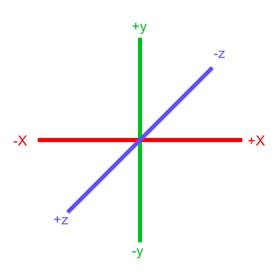
In the image above, the z-axis is considered positive when it's coming toward us and negative when it's going away from us. This convention uses the right-hand rule. Using your right hand, you point your thumb to the right, index finger straight up, and your middle finger toward you such that each of your three fingers are pointing in perpendicular directions like a coordinate system. Each finger is pointing in the positive direction.

You'll sometimes see this convention reversed along the z-axis when you're reading other peoples' code or reading other tutorials online. They might make the z-axis positive when it's going away from you and negative when it's coming toward you, but the x-axis and y-axis remain unchanged. This is known as the left-hand rule.

Ray Algorithms

Let's finally talk about "ray algorithms" such as ray marching and ray tracing. Ray marching is the most common algorithm used to develop 3D scenes in Shadertoy, but you'll see people leverage ray tracing or path tracing as well.

Both ray marching and ray tracing are algorithms used to draw 3D scenes on a 2D screen using rays. In real life, light sources such as the sun casts light rays in the form of photons in tons of different directions. When a photon hits an object, the energy is absorbed by the object's crystal lattice of atoms, and another photon is released. Depending on the crystal structure of the material's atomic lattice, photons can be emitted in a random direction (diffuse reflection), or at the same angle it entered the material (specular or mirror-like reflection).

I could talk about physics all day, but what we care about is how this relates to ray marching and ray tracing. Well, if we tried modelling a 3D scene starting at a light source and tracing it back to the camera, then we'd end up with a waste of computational resources. This "forward" simulation would lead to a ton of those rays never hitting our camera.

You'll mostly see "backward" simulations where rays are shot out of a camera or "eye" instead. We work backwards! Light usually comes from a light source such as the sun, bounces off a bunch of objects, and hits our camera. Instead, our camera will shoot out rays in lots of different directions. These rays will bounce off objects in our scene, including a surface such as a floor, and some of them will hit a light source. If a ray bounces off a surface and hits an object instead of the light source, then it's considered a "shadow ray" and tells us that we should draw a dark colored pixel to represent a shadow.

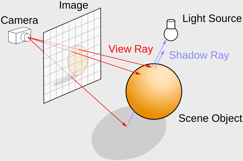
In the image above, a camera shoots out rays in different directions. How many rays? One for each pixel in our canvas! We use each pixel in the Shadertoy canvas to generate a ray. Clever, right? Each pixel has a coordinate along the x-axis and y-axis, so why not use them to create rays with a z-component?

How many different directions will there be? One for each pixel as well! This is why it's important to understand how rays work.

The ray origin for each ray fired from the camera will be the same as the position of our camera. Each ray will have a ray direction with an x-component, y-component, and z-component. Notice where the shadow rays originate from. The ray origin of the shadow rays will be equal to the point where the camera ray hit the surface. Every time the ray hits a surface, we can simulate a ray "bounce" or reflection by generating a new ray from that point. Keep this in mind later when we talk about illumination and shadows.

Difference between Ray Algorithms

Let's discuss the difference between all the ray algorithms you might see out there online. These include ray casting, ray tracing, ray marching, and path tracing.

Ray Casting: A simpler form of ray tracing used in games like Wolfenstein 3D and Doom that fires a single ray and stops when it hits a target.

Ray Marching: A method of ray casting that uses signed distance fields (SDF) and commonly a sphere tracing algorithm that "marches" rays incrementally until it hits the closest object.

Ray Tracing: A more sophisticated version of ray casting that fires off rays, calculates ray-surface intersections, and recursively creates new rays upon each reflection.

Path Tracing: A type of ray tracing algorithm that shoots out hundreds or thousands of rays per pixel instead of just one. The rays are shot in random directions using the Monte Carlo method, and the final pixel color is determined from sampling the rays that make it to the light source.

If you ever see "Monte Carlo" anywhere, then that tells you right away you'll probably be dealing with math related to probability and statistics.

You may also hear ray marching sometimes called "sphere tracing." There is a good discussion about the difference between ray marching and sphere tracing on the computer graphics Stack Exchange. Basically, sphere tracing is one type of implementation of ray marching. Most of the ray marching techniques you see on Shadertoy will use sphere tracing, which is still a type of ray marching algorithm.

In case you're wondering about spelling, I commonly see people use "raymarching" or "raytracing" as one word. When you're googling for resources on these topics or using Cmd+F (or Ctrl+F) to search for any reference of ray marching or ray tracing, keep this in mind.

Ray Marching

For the rest of this article, I'll be discussing how to use the ray marching algorithm in Shadertoy. There are many excellent online tutorials that teach about ray marching such as this tutorial by Jamie Wong. To help you visualize ray marching and why it's sometimes called sphere tracing, this tutorial on Shadertoy is a valuable resource.

I'll help break down the process of ray marching step by step, so you can start creating 3D scenes even with very little computer graphics experience.

We'll create a simple camera so we can simulate a 3D scene in the Shadertoy canvas. Let's imagine what our scene will look like first. We'll start with the most basic object: a sphere.

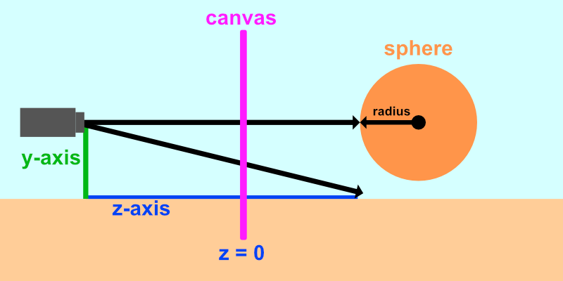
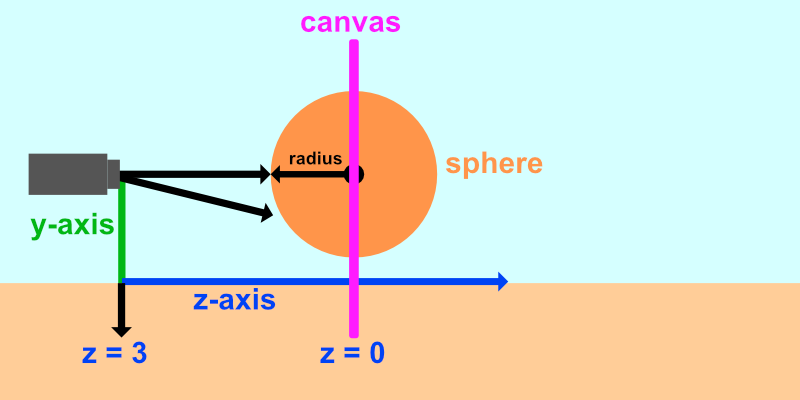
The image above shows a side view of the 3D scene we'll be creating in Shadertoy. The x-axis is not pictured because it is pointing toward the viewer. Our camera will be treated as a point with a coordinate such as (0, 0, 5) which means it is 5 units away from the canvas along the z-axis. Like previous tutorials, we'll remap the UV coordinates such that the origin is at the center of the canvas.

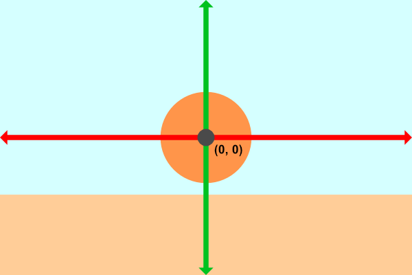
The image above represents the canvas from our perspective with an x-axis (red) and y-axis (green). We'll be looking at the scene from the view of the camera. The ray shooting straight out of the camera through the origin of the canvas will hit our sphere. The diagonal ray fires from the camera at an angle and hits the ground (if it exists in the scene). If the ray doesn't hit anything, then we'll render a background color.

Now that we understand what we're going to build, let's start coding! Create a new Shadertoy shader and replace the contents with the following to setup our canvas:

void mainImage( out vec4 fragColor, in vec2 fragCoord )
{
  vec2 uv = fragCoord/iResolution.xy; // <0, 1>
  uv -= 0.5; // <-0.5,0.5>
  uv.x *= iResolution.x/iResolution.y; // fix aspect ratio

  vec3 col = vec3(0);

  // Output to screen
  fragColor = vec4(col,1.0);
}

To make our code cleaner, we can remap the UV coordinates in a single line instead of 3 lines. We're used to what this code does by now!

void mainImage( out vec4 fragColor, in vec2 fragCoord )
{
  vec2 uv = (fragCoord - .5 * iResolution.xy) / iResolution.y; // Condense 3 lines down to a single line!

  vec3 col = vec3(0);

  // Output to screen
  fragColor = vec4(col,1.0);
}

The ray origin, ro will be the position of our camera. We'll set it 5 units behind the "canvas" we're looking through.

vec3 ro = vec3(0, 0, 5);

Next, we'll add a ray direction, rd, that will change based on the pixel coordinates. We'll set the z-component to -1 so that each ray is fired toward our scene. We'll then normalize the entire vector.

vec3 rd = normalize(vec3(uv, -1));

We'll then setup a variable that returns the distance from the ray marching algorithm:

float d = rayMarch(ro, rd, 0., 100.);

Let's create a function called rayMarch that implements the ray marching algorithm:

float rayMarch(vec3 ro, vec3 rd, float start, float end) {
  float depth = start;

  for (int i = 0; i < 255; i++) {
    vec3 p = ro + depth * rd;
    float d = sdSphere(p, 1.);
    depth += d;
    if (d < 0.001 || depth > end) break;
  }

  return depth;
}

Let's examine the ray marching algorithm a bit more closely. We start with a depth of zero and increment the depth gradually. Our test point is equal to the ray origin (our camera position) plus the depth times the ray direction. Remember, the ray marching algorithm will run for each pixel, and each pixel will determine a different ray direction.

We take the test point, p, and pass it to the sdSphere function which we will define as:

float sdSphere(vec3 p, float r)
{
  return length(p) - r; // p is the test point and r is the radius of the sphere
}

We'll then increment the depth by the value of the distance returned by the sdSphere function. If the distance is within 0.001 units away from the sphere, then we consider this close enough to the sphere. This represents a precision. You can make this value lower if you want to make it more accurate.

If the distance is greater than a certain threshold, 100 in our case, then the ray has gone too far, and we should stop the ray marching loop. We don't want the ray to continue off to infinity because that's a waste of computational resources and would make a for loop run forever if the ray doesn't hit anything.

Finally, we'll add a color depending on whether the ray hit something or not:

if (d > 100.0) {
  col = vec3(0.6); // ray didn't hit anything
} else {
  col = vec3(0, 0, 1); // ray hit something
}

Our finished code should look like the following:

float sdSphere(vec3 p, float r )
{
  return length(p) - r;
}

float rayMarch(vec3 ro, vec3 rd, float start, float end) {
  float depth = start;

  for (int i = 0; i < 255; i++) {
    vec3 p = ro + depth * rd;
    float d = sdSphere(p, 1.);
    depth += d;
    if (d < 0.001 || depth > end) break;
  }

  return depth;
}

void mainImage( out vec4 fragColor, in vec2 fragCoord )
{
  vec2 uv = (fragCoord-.5*iResolution.xy)/iResolution.y;

  vec3 col = vec3(0);
  vec3 ro = vec3(0, 0, 5); // ray origin that represents camera position
  vec3 rd = normalize(vec3(uv, -1)); // ray direction

  float d = rayMarch(ro, rd, 0., 100.); // distance to sphere

  if (d > 100.0) {
    col = vec3(0.6); // ray didn't hit anything
  } else {
    col = vec3(0, 0, 1); // ray hit something
  }

  // Output to screen
  fragColor = vec4(col, 1.0);
}

We seem to be reusing some numbers, so let's set some constant global variables. In GLSL, we can use the const keyword to tell the compiler that we don't plan on changing these variables:

const int MAX_MARCHING_STEPS = 255;
const float MIN_DIST = 0.0;
const float MAX_DIST = 100.0;
const float PRECISION = 0.001;

Alternatively, we can also use preprocessor directives. You may see people use preprocessor directives such as #define when they are defining constants. An advantage of using #define is that you're able to use #ifdef to check if a variable is defined later in your code. There are differences between #define and const, so choose which one you prefer and which ones works best for your scenario.

If we rewrote the constant variables to use the #define preprocessor directive, then we'd have the following:

#define MAX_MARCHING_STEPS 255
#define MIN_DIST 0.0
#define MAX_DIST 100.0
#define PRECISION 0.001

Notice that we don't use an equals sign or include a semicolon at the end of each line that uses a preprocessor directive.

The #define keyword lets us define both variables and functions, but I prefer to use const instead because of type safety.

Using these constant global variables, the code should now look like the following:

const int MAX_MARCHING_STEPS = 255;
const float MIN_DIST = 0.0;
const float MAX_DIST = 100.0;
const float PRECISION = 0.001;

float sdSphere(vec3 p, float r )
{
  return length(p) - r;
}

float rayMarch(vec3 ro, vec3 rd, float start, float end) {
  float depth = start;

  for (int i = 0; i < MAX_MARCHING_STEPS; i++) {
    vec3 p = ro + depth * rd;
    float d = sdSphere(p, 1.);
    depth += d;
    if (d < PRECISION || depth > end) break;
  }

  return depth;
}

void mainImage( out vec4 fragColor, in vec2 fragCoord )
{
  vec2 uv = (fragCoord-.5*iResolution.xy)/iResolution.y;

  vec3 col = vec3(0);
  vec3 ro = vec3(0, 0, 5); // ray origin that represents camera position
  vec3 rd = normalize(vec3(uv, -1)); // ray direction

  float d = rayMarch(ro, rd, MIN_DIST, MAX_DIST); // distance to sphere

  if (d > MAX_DIST) {
    col = vec3(0.6); // ray didn't hit anything
  } else {
    col = vec3(0, 0, 1); // ray hit something
  }

  // Output to screen
  fragColor = vec4(col, 1.0);
}

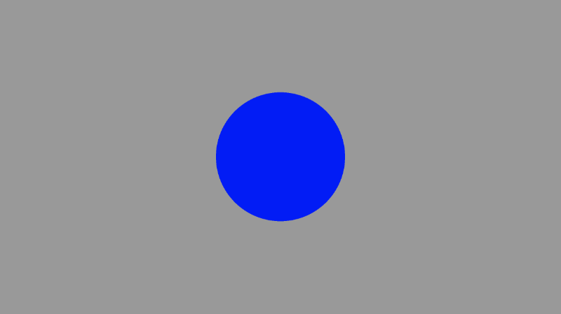
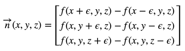
When we run the code, we should see an image of a sphere. It looks like a circle, but it's definitely a sphere!

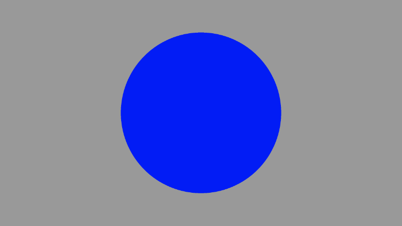
If we change the position of the camera, we can zoom in and out to prove that we're looking at a 3D object. Increasing the distance between the camera and the virtual canvas in our scene from 5 to 3 should make the sphere appear bigger as if we stepped forward a bit.

vec3 ro = vec3(0, 0, 3); // ray origin

There is one issue though. Currently, the center of our sphere is at the coordinate, (0, 0, 0) which is different than the image I presented earlier. Our scene is setup that the camera is very close to the sphere.

Let's add an offset to the sphere similar to what we did with circles in Part 2 of my tutorial series.

float sdSphere(vec3 p, float r )
{
  vec3 offset = vec3(0, 0, -2);
  return length(p - offset) - r;
}

This will push the sphere forward along the z-axis by two units. This should make the sphere appear smaller since it's now farther away from the camera.

Lighting

To make this shape look more like a sphere, we need to add lighting. In the real world, light rays are scattered off objects in random directions.

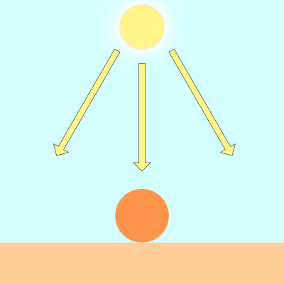
Objects appear differently depending on how much they are lit by a light source such as the sun.

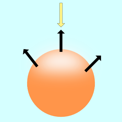
The black arrows in the image above represent a few surface normals of the sphere. If the surface normal points toward the light source, then that spot on the sphere appears brighter than the rest of the sphere. If the surface normal points completely away from the light source, then that part of the sphere will appear darker.

There are multiple types of lighting models used to simulate the real world. We'll look into Lambert lighting to simulate diffuse reflection. This is commonly done by taking the dot product between the ray direction of a light source and the direction of a surface normal.

vec3 diffuseReflection = dot(normal, lightDirection);

A surface normal is commonly a normalized vector because we only care about the direction. To find this direction, we need to use the gradient. The surface normal will be equal to the gradient of a surface at a point on the surface.

Finding the gradient is like finding the slope of a line. You were probably told in school to memorize the phrase, "rise over run." In 3D coordinate space, we can use the gradient to find the "direction" a point on the surface is pointing.

If you've taken a Calculus class, then you probably learned that the slope of a line is actually just an infinitesimally small difference between two points on the line.

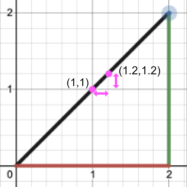
Let's find the slope by performing "rise over run":

Point 1 = (1, 1)
Point 2 = (1.2, 1.2)

Rise / Run = (y2 - y1) / (x2 - x1) = (1.2 - 1) / (1.2 - 1) = 0.2 / 0.2 = 1

Therefore, the slope is equal to one.

To find the gradient of a surface, we need two points. We'll take a point on the surface of the sphere and subtract a small number from it to get the second point. That'll let us perform a cheap trick to find the gradient. We can then use this gradient value as the surface normal.

Given a surface, f(x,y,z), the gradient along the surface will have the following equation:

The curly symbol that looks like the letter, "e", is the greek letter, epsilon. It will represent a tiny value next to a point on the surface of our sphere.

In GLSL, we'll create a function called calcNormal that takes in a sample point we get back from the rayMarch function.

vec3 calcNormal(vec3 p) {
  float e = 0.0005; // epsilon
  float r = 1.; // radius of sphere
  return normalize(vec3(
    sdSphere(vec3(p.x + e, p.y, p.z), r) - sdSphere(vec3(p.x - e, p.y, p.z), r),
    sdSphere(vec3(p.x, p.y + e, p.z), r) - sdSphere(vec3(p.x, p.y - e, p.z), r),
    sdSphere(vec3(p.x, p.y, p.z  + e), r) - sdSphere(vec3(p.x, p.y, p.z - e), r)
  ));
}

We can actually use Swizzling and vector arithmetic to create an alternative way of calculating a small gradient. Remember, our goal is to create a small gradient between two close points on the surface of the sphere (or approximately on the surface of the sphere). Although this new approach is not exactly the same as the code above, it works quite well for creating a small value that approximately points in the direction of the normal vector. That is to say, it works well at creating a gradient.

vec3 calcNormal(vec3 p) {
  vec2 e = vec2(1.0, -1.0) * 0.0005; // epsilon
  float r = 1.; // radius of sphere
  return normalize(
    e.xyy * sdSphere(p + e.xyy, r) +
    e.yyx * sdSphere(p + e.yyx, r) +
    e.yxy * sdSphere(p + e.yxy, r) +
    e.xxx * sdSphere(p + e.xxx, r));
}

The important thing to realize is that the calcNormal function returns a ray direction that represents the direction a point on the sphere is facing.

Next, we need to make a position for the light source. Think of it as a tiny point in 3D space.

vec3 lightPosition = vec3(2, 2, 4);

For now, we'll have the light source always pointing toward the sphere. Therefore, the light ray direction will be the difference between the light position and a point we get back from the ray march loop.

vec3 lightDirection = normalize(lightPosition - p);

To find the amount of light hitting the surface of our sphere, we must calculate the dot product. In GLSL, we use the dot function to calculate this value.

float dif = dot(normal, lightDirection); // dif = diffuse reflection

When we take the dot product between the normal and light direction vectors, we may end up with a negative value. To keep the value between zero and one so that we get a bigger range of values, we can use the clamp function.

float dif = clamp(dot(normal, lightDirection), 0., 1.);

Putting this altogether, we end up with the following code:

const int MAX_MARCHING_STEPS = 255;
const float MIN_DIST = 0.0;
const float MAX_DIST = 100.0;
const float PRECISION = 0.001;

float sdSphere(vec3 p, float r )
{
  vec3 offset = vec3(0, 0, -2);
  return length(p - offset) - r;
}

float rayMarch(vec3 ro, vec3 rd, float start, float end) {
  float depth = start;

  for (int i = 0; i < MAX_MARCHING_STEPS; i++) {
    vec3 p = ro + depth * rd;
    float d = sdSphere(p, 1.);
    depth += d;
    if (d < PRECISION || depth > end) break;
  }

  return depth;
}

vec3 calcNormal(vec3 p) {
    vec2 e = vec2(1.0, -1.0) * 0.0005; // epsilon
    float r = 1.; // radius of sphere
    return normalize(
      e.xyy * sdSphere(p + e.xyy, r) +
      e.yyx * sdSphere(p + e.yyx, r) +
      e.yxy * sdSphere(p + e.yxy, r) +
      e.xxx * sdSphere(p + e.xxx, r));
}

void mainImage( out vec4 fragColor, in vec2 fragCoord )
{
  vec2 uv = (fragCoord-.5*iResolution.xy)/iResolution.y;

  vec3 col = vec3(0);
  vec3 ro = vec3(0, 0, 3); // ray origin that represents camera position
  vec3 rd = normalize(vec3(uv, -1)); // ray direction

  float d = rayMarch(ro, rd, MIN_DIST, MAX_DIST); // distance to sphere

  if (d > MAX_DIST) {
    col = vec3(0.6); // ray didn't hit anything
  } else {
    vec3 p = ro + rd * d; // point on sphere we discovered from ray marching
    vec3 normal = calcNormal(p);
    vec3 lightPosition = vec3(2, 2, 4);
    vec3 lightDirection = normalize(lightPosition - p);

    // Calculate diffuse reflection by taking the dot product of
    // the normal and the light direction.
    float dif = clamp(dot(normal, lightDirection), 0., 1.);

    col = vec3(dif);
  }

  // Output to screen
  fragColor = vec4(col, 1.0);
}

When you run this code, you should see a lit sphere! Now, you know I was telling the truth. Definitely looks like a sphere now! 😁

If you play around with the lightPosition variable, you should be able to move the light around in the 3D world coordinates. Moving the light around should affect how much shading the sphere gets. If you move the light source behind the camera, you should see the center of the sphere appear a lot brighter.

vec3 lightPosition = vec3(2, 2, 7);

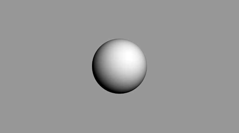
You can also change the color of the sphere by multiplying the diffuse reflection value by a color vector:

col = vec3(dif) * vec3(1, 0.58, 0.29);

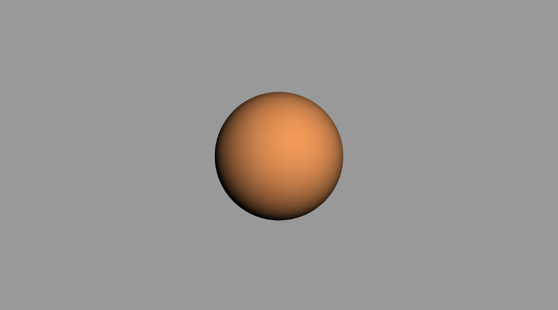
If you want to add a bit of ambient light color, you can adjust the clamped range, so the sphere doesn't appear completely black in the shaded regions:

float dif = clamp(dot(normal, lightDirection), 0.3, 1.);

You can also change the background color and add a bit of this color to the color of the sphere, so it blends in well. Looks a bit like the reference image we saw earlier in this tutorial, huh? 😎

For reference, here is the completed code I used to create the image above.

const int MAX_MARCHING_STEPS = 255;
const float MIN_DIST = 0.0;
const float MAX_DIST = 100.0;
const float PRECISION = 0.001;

float sdSphere(vec3 p, float r )
{
  vec3 offset = vec3(0, 0, -2);
  return length(p - offset) - r;
}

float rayMarch(vec3 ro, vec3 rd, float start, float end) {
  float depth = start;

  for (int i = 0; i < MAX_MARCHING_STEPS; i++) {
    vec3 p = ro + depth * rd;
    float d = sdSphere(p, 1.);
    depth += d;
    if (d < PRECISION || depth > end) break;
  }

  return depth;
}

vec3 calcNormal(vec3 p) {
    vec2 e = vec2(1.0, -1.0) * 0.0005; // epsilon
    float r = 1.; // radius of sphere
    return normalize(
      e.xyy * sdSphere(p + e.xyy, r) +
      e.yyx * sdSphere(p + e.yyx, r) +
      e.yxy * sdSphere(p + e.yxy, r) +
      e.xxx * sdSphere(p + e.xxx, r));
}

void mainImage( out vec4 fragColor, in vec2 fragCoord )
{
  vec2 uv = (fragCoord-.5*iResolution.xy)/iResolution.y;
  vec3 backgroundColor = vec3(0.835, 1, 1);

  vec3 col = vec3(0);
  vec3 ro = vec3(0, 0, 3); // ray origin that represents camera position
  vec3 rd = normalize(vec3(uv, -1)); // ray direction

  float d = rayMarch(ro, rd, MIN_DIST, MAX_DIST); // distance to sphere

  if (d > MAX_DIST) {
    col = backgroundColor; // ray didn't hit anything
  } else {
    vec3 p = ro + rd * d; // point on sphere we discovered from ray marching
    vec3 normal = calcNormal(p);
    vec3 lightPosition = vec3(2, 2, 7);
    vec3 lightDirection = normalize(lightPosition - p);

    // Calculate diffuse reflection by taking the dot product of
    // the normal and the light direction.
    float dif = clamp(dot(normal, lightDirection), 0.3, 1.);

    // Multiply the diffuse reflection value by an orange color and add a bit
    // of the background color to the sphere to blend it more with the background.
    col = dif * vec3(1, 0.58, 0.29) + backgroundColor * .2;
  }

  // Output to screen
  fragColor = vec4(col, 1.0);
}

Conclusion

Phew! This article took about a weekend to write and get right, but I hope you had fun learning about ray marching! Please consider donating if you found this tutorial or any of my other past tutorials useful. We took the first step toward creating a 3D object using nothing but pixels on the screen and a clever algorithm. Til next time, happy coding!

Resources

• Difference between Ray Algorithms
• Ray Marching Tutorial by Jamie Wong
• Wikipedia: Ray Tracing
• Wikipedia: Lambertian Reflectance
• Wikipedia: Surface Normals
• Wolfram MathWorld: Gradient
• Wolfram MathWorld: Dot Product
• Shadertoy: Visual Ray Marching Tutorial
• Shadertoy: Super Simple Ray Marching Tutorial
• Shadertoy: Box and Balloon
• Shadertoy: Let's Make a Ray Marcher
• Shadertoy: Ray Marching Primitives
• Shadertoy: Ray Marching Sample Code
• Shadertoy: Ray Marching Template